mpirun -np 4 ./cosmomc params.ini

python python/runMPI.py params

If things go wrong check the .log and any error files in your cosmomc/scripts directory.

• Parameter limits and proposal density
  The parameter limits, estimated distribution widths and starting points are listed as the param[paramname] variables for each parameter, of the form

   param[paramname] = center min max start_width propose_width
  

  The start_width entry determines the randomly chosen dispersion of the starting position about the given centre, and should be as large or larger than the posterior (for the convergence diagnostic to be reliable, chains should start at widely separated points). Chains are restricted to stay within the bounds determined by min and max. If the parameter is not to be varied in your run, you can just specify the fixed value.

  The sampler proposes changes in parameters using a proposal density function with a width determined by propose_width (multiplied by the value of the global propose_scale parameter). The propose_width should be of the order of the conditional posterior width (i.e. the expected error in that parameter when other parameters are fixed). If you specify a propose_matrix (approximate covariance matrix for the parameters), the parameter distribution widths are determined from its eigenvalues instead, and the proposal density changes the parameter eigenvectors. The covariance matrix can be computed using "getdist" once you have done one run - the file_root.covmat file. The planck_covmats/ directory is supplied with many you can use. The covariance matrix does not have to include all the parameters that are used - zero entries will be updated from the input propose widths of new parameters (the propose width should be of the size of the conditional distribution of the parameter - typically quite a bit smaller than the marginalized posterior width; generally too small is better than too large). The scale of the proposal density relative to the covariance is given by the propose_scale parameter. If your propose_matrix is significantly broader than the expected posterior, this number can be decreased.

  If you don't have a propose_matrix, you can use estimate_propose_matrix = T to automatically estimate it by numerical fitting about the best fit point (with action=2 to stop, or action=0 to continue straight into an MCMC run).
  
  

• Sampling method
  Set sampling_method=1 to use a vanilla Metropolis algorithm (in the optimal fast/slow subspaces if use_fast_slow is true). Set sampling_method=7 to use a fast-slow dragging algorithm (Neal 2005), which allows fast nuisance parameters to be handled efficiently; this is the default for Planck runs.

  Other sampling methods that were implemented in previous version have not currently been updated for the latest version.

• CAMB's numerical accuracy
  The default accuracy is aimed at WMAP. Set high_accuracy_default = T to target ~0.1% accuracy on the CMB power spectra from CAMB. This is sufficient for numerical biases to be small compared to the error bar for Planck; for an accuracy study see arXiv:1201.3654. You can also use the accuracy_level parameter to increase accuracy further, however this is numerically inefficient and is best used mainly for numerical stability checks using importance sampling (action=1).
  
  
• Best-fit point
  Set action =2 to just calculate the best-fit point and stop. This uses Powell's 2009 BOBYQA bounded minimization routine, which works from two parameters up to hundreds of parameters, but does require that the likelihood return a valid number at all points between the bounds given on the base parameters in the input .ini file. The algorithm starts at the point given by the center parameter values given in the .ini file, and iterates until the parameter values are converged to within a radius of max_like_radius (in normalized units, e.g. fraction of a standard deviation or propose_width). The minimization will also stop if the log likelihood has converged to within minimize_loglike_tolerance. The best-fit values (and derived and nuisance parameters) are output to a file called file_root.minimum. The method works for parameters with hard bounds that truncate the posterior, e.g. for neutrino mass mnu>0.
  
  Minimization with action=2 will work more reliably if you have a propose_matrix to approximately orthogonalize the likelihood. You can also run minimizations from multiple random starting points to check that they converge: run with e.g. "mpirun -np 4" and minimize_random_start_pos=T to check four minimizations - the final output will be the point with the best fit of all and a warning will be printed if there there are outliers.
  
  
• Data file output
  Since consecutive points are correlated and the output files can get quite large, you may want to thin the chains automatically: set the indep_sample parameter to determine at what frequency full information is dumped to a binary .data file (which includes the Cls, matter power spectrum, parameters, etc). If zero no .data file is generated. You only need to keep nearly uncorrelated samples for later importance sampling. You can specify a burn_in, though you may prefer to set this to zero and remove entries when you come to process the output samples.
  
  
• Threads and run-time adjustment
  The num_threads parameter will determine the number of openMP threads (in MPI runs, usually set to the number of CPUs on each node). Scaling is linear up to about 8 processors on most systems, then falls off slowly. It is probably best to run several chains on 8 or fewer processors. You can terminate a run before it finishes by creating a file called file_root_NN.read containing "exit =1" - it will read it in, delete the .read file and stop. The .read file can also have "num_threads =xx" to change the number of threads (per chain) dynamically. If you have multiple chains you can create file_root.read which will be read by all the chains. In this case the .read file is not deleted automatically.
  
  
• Post-processing (e.g. importance sampling)
  The action variable determines what to do. Use action=1 to process a .data file produced by a previous MCMC run - this is used for importance sampling with new data, correcting results generated by approximate means, or re-calculating the theoretical predictions in more detail. If action=1 set the redo_xxx parameters to determine what to do. With redo_add=F you should include all the data you want used for the final result (e.g. if you generated original samples with CMB data, also include CMB data when you importance sample - it will not be weighted twice). With redo_add=T you should include only data you want to add - the new likelihoods are added to those already stored in the chains. PostProcessing is fastest if you have binary .data files from an original run, however if you do not have these you can use redo_from_text=T to read in chains from .txt files.
  
  
• Exploring tails and high-significant limits
  The temperature setting allows you to sample from P^(1/T) rather than P - this is good for exploring the tails of distributions, discovering other local minima, and for getting more robust high-confidence error bars. See also the different sampling_methods.
  
  
• Checkpointing
  Set checkpoint = T in the .ini file to checkpoint: i.e. generate files so that if the processes are terminated they can be restarted again from close to where they left off. With MPI this setting creates file_root.chk files used to store the current status. To continue a prematurely terminated run, just run again using exactly the same commands and files as originally. Note that if you use checkpointing, but you want to overwrite existing chains of the same name, you must manually delete all the file_root.* files (otherwise it will attempt to continue from where they left off). Please note this feature is not fantastically well tested, please let us know of any problems. Also note that for checkpointing to work the first run must run for at least past the initial burn phase (you can see when the file_root.chk files have been produced), otherwise the run will just start from scratch again.

The runMPI.py and runbatch.py submission scripts use a job template file to submit jobs to the queue on your cluster. The job_script files is supplied as sample, and you may need to make your own template specific to the configuration of your machine, depending on what queuing system you have (e.g. PBS, SLURM, etc.) Recommended steps are

• If necessary, copy job_script to a new file, e.g. job_script_mycluster which you will then edit
• If necessary, edit the template script:
  • Things of the form ##tag## are placeholders, and are replaced by relevant values for each run. Leave these as is, just edit the surrounding text so they are put in the right places.
  • The line starting ##RUN: gives the template for each mpirun command used to actually run jobs.
  • Lines of the form ##DEFAULT_xxx: yyy ## give names of specific commands or settings on your machine, for example ##DEFAULT_qsub: msub ## sets the job submission command to "qsub".
• Set COSMOMC_xxx environment variable in your .bashrc to give the name of the script template filename, and any other job setting defaults that you want to override from the job template used. E.g.

  export COSMOMC_job_template=job_script_mycluster
  export COSMOMC_coresPerNode=8
  export COSMOMC_nodes=2
  export COSMOMC_chainsPerNode=2
  export COSMOMC_queue=default_queue
  export COSMOMC_walltime=24:00:00
  

• Using the python/GetDist.py program (which can be run without having a fortran compiler installed).
• With the GetDist Gui interactive program, in python/GetDistGUI.py. See the GetDist GUI readme.
• Programmatically, using the python modules via python scripts.
• Using the getdist program, compiled with Fortran (used by Planck 2015 chains, but now deprecated)

xxx_1.txt
xxx_2.txt
...
xxx.paramnames
xxx.ranges

    weight like param1 param2 param3 ...

The weight gives the number of samples (or importance weight) with these parameters. like gives -log(likelihood), and param1, param2... are the values of the parameters at each point.

The .paramnames file lists the names of the parameters, one per line, optionally followed by a latex label. Names cannot include spaces, and if they end in "*" they are interpreted as derived (rather than MCMC) parameters, e.g.

x1   x_1
y1   y_1
x2   x_2
xy*  x_1+y_1

x1  -5 5
x2   0 N

The GetDist program, scripts and gui could be used completely independently of the CosmoMC program if you produce chains (or samples) in the same format (see the pip-installable python package). If there is just one file of samples, you can also use xxx.txt without the _n number tag that's used to denote separate chains.

Running the GetDist program

Running using the python version

python python/GetDist.py [distparams.ini] [chains/chainroot]

./getdist distparams.ini [chains/chainroot]

python python/GetDist.py --make_param_file myparams.ini

Note that the outputs from the python and fortran versions of GetDist are not identical due to slightly different algorithms, but should usually be consistent to better than the sampling noise for parameter means and limits. Both can produce pre-computed densities for plotting (in the plot_data_dir directory), but the python plotting scripts do not require this - output will be faster and make far fewer files if plot_data_dir is not set.

GetDist Parameters

• GetDist processes the file_root.txt file, and outputs statistics, marginalized plots, samples plots, and performs PCA (principle component analysis).
  
  
• Set ignore_rows to a positive integer to ignore that number of output rows as burn-in, or to a fraction <1 to skip that fraction of each chain's rows.
  
  
• Set the parameter_names parameter to specify a .paramnames file with the names and labels for parameters corresponding to the various columns in the chain files (see the supplied examples). If this parameter is empty getdist reads the parameters from the file_root.paramnames file that is output when generating the chains.
  
  
• If you have a derived parameter which has a prior which cuts off when the posterior is non-negligible you need to either set the limits in a xxx.derived_ranges file analogous to the xxx.paramnames file being when running the chains, or set the limits[paramname] variables to the corresponding limits when running GetDist. Otherwise limits are computed automatically. DO NOT use limits[paramname] to change the bounds on other plots - the program uses the limits information when it is estimating the posteriors from the samples. Limits for base MCMC and standard derived parameters are set automatically from the .ranges file produced with the chain. If only one end is fixed you can use N the floating end, e.g. "limitsxx = 0 N" for the tensor amplitude which has a greater than zero prior.

  Example: Since often people get this wrong with new parameters, here is an illustration of what happens when generating plots from a tensor run set of chains (with prior r>0):

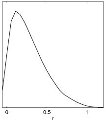
  Incorrect result when no chain.ranges file and limits[r02] is not set.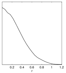

  Correct result when setting limits[r02]=0 N (or using default .ranges file, which includes the equivalent prior information from paramnames/derived_tensors.derived_ranges).

  Various parameters determine how sample densities are computed (see the Kernel Density Estimation notes). The smooth_scale_1D and smooth_scale_2D parameters can be set to change the smoothing scale. For smooth_scale_1D:

  • if smooth_scale_1D >= 1 smooth by smooth_scale_1D bin widths
  • if smooth_scale_1D> 0 and <1 smooth by Gaussian of smooth_scale_1D standard deviations in each parameter (around 0.2-0.3 is often good); this gets flat distributions nice and smooth without overly broadening well determined parameters
  • if smooth_scale_1D< 0 uses automatic smoothing length (changes with parameter)-the overall smoothing length is scaled by abs(smooth_scale_1D) from very crude guess at best overall scale

  The behaviour for smooth_scale_2D is similar. Usually the default =-1 setting can be used, which choose smoothing automatically, but changing it can be a good way to enforce a smaller smoothing scale (for example if you have too few samples, the auto-scaling will make the smoothing relatively large, which can sometimes make the results somewhat artificially better than they really are).

Output Text Files
These are all output by the GetDist program, and most can also be viewed on demand by using the menu options in the GetDist GUI.

• file_root.margestats file contains the means, standard deviations and marginalized limits for the different parameters (including derived parameters). Limits to calculate are set using the contourxx input parameters.
  
  
• file_root.likestats gives the best fit sample model, its likelihood, and limits from the extremal values of the N-dimensional distribution. Note that MCMC does not generally provide accurate values for the best-fit.
  
  
• file_root.converge contains various convergence diagnostics
  
  
• file_root.PCA contains a principle component analysis (PCA) for PCA_num parameters, specified in PCA_params parameter. You can specify the mapping used with PCA_func, for example 'L' to use logs (what you usually want for positive definite parameters). The output file contains the analysis including the correlation matrix, eigenvectors and eigenvalues, as well as the well constrained parameter combinations and their marginalized errors. This is how you automatically work out constraints of the form param1^a param2^b param3^c ...  = x \pm y.
  
  
• file_root.corr contains parameter correlations
  
  
• file_root.covmat contains a covariance matrix you can use as a proposal matrix for generating future chains
  
  

Plotting

GetDist can be used to produce basic simple scripts for various types of plots. You can also just write plotting scripts, or use the GetDist GUI, in which case there is no need to run GetDist first.

• Interactive plotting
  See the GetDist GUI readme for details of hope to use the GetDist GUI to make plots from chains. Even if you ultimately write custom scripts to optimize how things are displayed, this can be a quick and easy way to compare results and see what you want to plot.
• Python plot scripts
  See the CosmoMC python readme for details of how to use the plotting library.

If no_plots=F, GetDist produces scripts files to make simple 1D, 2D and 3D plots. The script files produced are called

• file_root for 1D marginalized plots
• file_root_2D for 2D marginalized plots
• file_root_3D to make coloured 2D samples plots
• file_root_tri to make 'triangle' plots (example. Set triangle_plot=T in the .ini file)

Parameter labels are set in distparams.ini - if any are blank the parameter is ignored. You can also specify which parameters to plot, or if parameters are not specified for the 2D plots or the colour of the 3D plots getdist automatically works out the most correlated variables and uses them. The data files used by auto-generated plotting scripts are output to the plot_data directory.

Convergence diagnostics

• For multiple chains the code computes the Gelman and Rubin "variance of chain means"/"mean of chain variances" R statistic for each parameter using the second half of each chain (reference). The .converge file produced by getdist contains the numbers for each parameter individually. The program also writes out the value for the worst eigenvalue of the covariance of the means, which should be a worst case (catching poor chain coverage in directions not aligned with the base parameters). This "R-1" statistic is also used for the stopping criterion when generating chains with MPI. If the numbers are much less than one then the second half of each chain probably provides an accurate estimate of the means and variances. If the distribution is bimodal and no chains find the second mode low values can be misleading. Typically you want the value to be less than 0.1, or lower if you want means to high accuracy or to make nice 2D density plots (0.01 is often fine). Low values do not guarantee that small percentiles will be measured accurately (though it certainly helps), or that the value won't increase as you run longer and probe further into the tails.
  
  
• For MPI runs, in addition to specifying a stopping criterion as above, you can also give a convergence criterion for a confidence limit. In general it is much harder to get an accurate value for a small confidence value than for the mean, so imposing a tight limit may make your chains run for a very long time (though you can then be pretty confident in your confidence). The value computed is the variance of the chain percentiles from the last half of the different chains, in units of the standard deviation of each parameter. You can either specify a particular parameter to check, or do all of them. Any parameter with a slowly explored tail will only converge very slowly, in which case you may be able to improve things by generating chains at a higher temperature (so the tails are explored more readily; GetDist can adjust for the temperature automatically), or re-parameterizing.
  
  
• The auto-correlation length gives a measure of how independent the samples are, with the total number of samples divided by the length giving an estimate of an effective number of independent samples. Two auto-correlation lengths are computed, in 'weight' units and 'sample' units. The latter is in units of the number of rows in the chain file, the former is the "weight mass' that determines the correlation length; for definitions see the GetDist notes.
  
  
• For individual chains (before importance sampling) getdist computes the Raftery and Lewis convergence diagnostics. This uses a binary chain derived from each parameter depending on whether the parameter is above or below a given percentile of its distribution (specified by the converge_test_limit input parameter). The code works out how much the binary chain needs to be thinned to approximate a Markov process better than a second order process, and then uses analytical results for the convergence of binary Markov chains to assess the burn in period. It also assesses the thin factor needed for the binary chain to approximate an independence chain, which gives an idea of how much you need to thin the chain to obtain independent samples (i.e. how much you can get away with thinning it for importance sampling, though thinning isn't entirely lossless). The .converge file contains the numbers for each chain used, getdist writes out the worst case. See this reference for details.
  
  
• A simpler way to assess the error on quantile limits is by computing them using subsets of the samples. GetDist produces the file_root.converge contains the 'split-test' rms change on the parameter quantiles in units of the standard deviation when the samples are split into 2,3 or 4 parts. Small numbers are clearly better. A number of 0.5 for a 2-way split indicates that the 95% confidence limit may in fact be off by the order of half a standard deviation (though probably better, as the limit is computed using all the samples). Large values in a particular parameter may indicate that there is a long tail that is only being explored slowly (in which case generating the chain at a higher temperature or changing parameters to the log might help).

Differences between GetDist and MPI run-time statistics

GetDist will cut out ignore_rows from the beginning of each chain, then compute the R statistic using all of the remaining samples. The MPI run-time statistic uses the last half of all of the samples. In addition, GetDist will use all the parameters, including derived parameters. If a derived parameter has poor convergence this may show up when running GetDist but not when running the chain (however the eigenvalues of covariance of means is computed using only base parameters). The run-time values also use thinned samples (by default every one in ten), whereas GetDist will use all of them. GetDist will allow you to use only subsets of the chains.

Likelihoods that you use may also have their own nuisance parameters.

Using CosmoMC as a generic sampler

• Write your own likelihood in GenericLikelihoodFunction in calclike.f90
• Adapt params_generic.ini appropriately for your parameter numbers and settings (see comments there)
• Run using your .ini file as normal

The code makes use of Fortran 2003 features and structures. There is automated code documentation, which includes modules, classes and subroutines. File and class documentation gives inheritance trees to help understand the structure, for example GeneralTypes.f90 contains the key base classes that other things are inherited from.

You are encouraged to examine what the code is doing and consider carefully changes you may wish to make. For example, the results can depend on the parameterization. You may also want to use different CAMB modules, e.g. slow-roll parameters for inflation, or use a fast approximator. The main source code files you may want to modify are

• settings.f90
This defines the maximum number of parameters and their types.
• Calculator_Cosmology.f90 and Calculator_CAMB.f90
Routines for generating Cls, matter power spectra and sigma8 from CAMB. Override the calcualtor class in Calculator_Cosmology.f90 to implement cosmology using other calculatorse.g. a fast approximator like PICO, or other Boltzmann code. etc.
• DataLikelihoods.f90
This is where you can add in new likelihood functions
• driver.F90
Main program that reads in parameters and calls MCMC or post-processing.
• propose.f90
This is the proposal density and related constants and subroutines. The efficiency of MCMC is quite dependent on the proposal. Fast+slow and fast parameter subspaces are proposed separately. See the paper for a discussion of the proposal density and use of fast and slow parameters.

• CosmoChord (and PolyChord, Next Generation Nested Sampler)
• Integrated Software in Testing General Relativity (ISiTGR)
• fgas (Relaxed Galaxy Clusters, available as clusters_fgas branch in git repository)

• June 2021
  
  • Updated to CAMB version 1.3.2
  • Updated to GetDist 1.3
  • Fix for output of tensor derived parameters
  • Add CamSpec files
  • Minor bug fixes
• May 2020
  
  • Updated to CAMB version 1.1.2
  • Updated to GetDist 1.0 (removing obsolete fortran version).
  • Fix for using astro parameterization output thinning
• July 2019
  
  • Added Planck 2018 likelihoods and associated files.
  • Minor updated Pantheon (batch3/Pantheon18.ini)
  • batch3/HST_Riess19.ini for latest H0
  • Add DR14 Lyman-alpha BAO (thanks Pablo-Lemos)
  • Bug fixes and misc compatibility improvements
  • Updated to latest GetDist
  • GetDist GUI supports Python 3 with PySide2
  • Make Planck2018 branch for fixed version consistent with that used for release (uses CAMB July 2018)
  • Updated to CAMB version 1.0.7. (note that this changes likelihood values slightly compared to Planck2018 branch; also HMcode version changes for numerical stability and speed)
• October 2018
  
  • Added DES 1 Yr data (batch3/DES.ini and variants, likelihood is implemented natively in wl.f90)
  • Added BICEP-Keck 2015 likelihood and data (batch3/BK15.ini)
  • Misc updates to CAMB and getdist (see github history)
  • Fix bug settings nnu<3.046 and degenerate neutrino masses
  • Fixed gfortran issue with checkpointing
• July 2018
  
  • Added Planck 2018 lensing likelihoods (batch3/lensing.ini and batch3/lensonly.ini)
  • Added Riess et al. SH0ES H_0 constraints in (in batch3/)
  • New wl.f90 for galaxy lensing and cross-correlations (actual DES likelihood files not provided until published)
  • batch3/ .ini files settings for Planck 2018 runs (excluding 2018 CMB likelihoods which are not released yet)
  • Added element abundance likelihoods and new BBN interpolation grids for Parthenope and PRIMAT codes
  • Added SPT-SZ 2500d TT (thanks Christian Reichardt)
  • CMBlikes now supports aberration correction parameter (thanks Christian Reichardt)
  • Added BAO consensus: batch3/DR12_BAO_consensus.ini and batch3/DR12_FS_consensus.ini. BAO module updated to support DM measurements, measurement files without error columns, reading either covariance or inverse covariance, support for multiple specified zeff.
  • Python grids now have getdist_options dictionary to specify grid-level getdist parameters (so now no batch3 equivalent of batch2/getdist_common.ini)
  • Parameter grids support python filters functions that act over all chains (e.g. to import z_re<6.5 prior) and partial support for recursive importance sampling (only filtering)
  • Built-in support for power-law extrapolation of matter power P(k) beyond kmax to extrap_kmax (700h/Mpc by default)
  • added "astro" parameterization using flat prior in H0, omegam, omegab, logA
  • Fixed output of first sample when importance sampling with redo_skip
  • Importance sampled chains with redo_skip now produce .properties.ini to flag chain as burn-removed
  • CMBlikes optimizations and fixes. BKP nuisance parameters now used as fast parameters.
  • GetDist changes:
    • Improvements to triangle_plot for the upper triangle
    • get_axes_for_params() function for easier post-manipulation of axes
    • plots now support MixtureND instances for plotting Gaussian mixture models directly (or just GaussianND, Gaussian2D)
    • plots add_2D_covariance function to directly plot contours from given mean and covariance
    • add_2D_mixture_projection function to plot specific 2D marginalized contours for MixtureND Gaussian mixture
    • settings parameters: auto_ticks whether to use matplotlib 2 'auto' tick numbering (does not work well for grids of plots, default: False);
    • thin_long_subplot_ticks, whether to try to prevent x-axis label overlap when long numbers in tick labels (default: True)
    • samples getParamSampleDict() function to get dictionary of parameter values for given sample number
    • samples saveChainsAsText() function to re-save set of chain files (with ranges and names)
    • gaussian_mixtures classes now have paramNames, and getUpper/getLower functions for easier integration with plotting scripts; GaussianND convenience special-case class.
    • paramNames can now be instantiated with list of labels (rather than having to call separate function)
    • ParamBounds fixedValue and fixedValueDict functions to get fixed parameter values
    • alpha_scatter option to _3d plots, to plot all samples alphaed by their weights
    • Better support for reading nested-sampling chains: now ignores all samples with weight less than min_weight_ratio=1e-30 of the maximum weight
    • MCSamples.addDerived() function now supports specification of parameter range
    • Various misc fixes
• November 2016
  
  • Added .derived_ranges files (in /paramnames folder) to specify hard priors on derived parameters. These are now propagated to output chain .ranges file along with H0 and z_rei priors (and hence limits do not need to be manually specified when running GetDist).
  • Added neutrino_hierarchy (={normal, inverted, degenerate}), to support one or two distinct eigenstate approximation to oscillation constraints.
  • python/runGridGetDist.py script now uses python getdist. Batch3-based grids no longer use getdist_common.ini, but default getdist settings (+ what's set in the grid setting file).
  • Bicep BK14 data files and CMB_BK_Planck update (thanks Colin Bischoff)
  • Support for BAO .dataset files with no measurement_type keyword (set in data file for each point instead)
  • Updated getdist to 0.2.6 (fixing compatibility issue with latest matplotlib for 2D contours)
  • Update CAMB to Nov 2016 version
• June 2016
  
  • CAMB updated to May 2016 version (including HMCode Halofit support)
  • Added DR12 BAO (in batch3/, thanks Tom Charnock)
  • Added batch3/HST_Riess2016.ini
  • Added include_fixed_parameter_priors input option (default false, as before)
  • Latest GetDist version and small fixes
• July 2015
  
  • Data Updates:
    • Settings (batch2/) for the Planck 2015 likelihood release. Planck lensing and BKP likelihoods are native and included with cosmomc, others can be linked to the Planck likelihood code.
    • Added SZ likelihood, szcounts.f90, as used by the Planck 2015 cluster paper
    • BKP likelihood update to include tests including E; small fix to covariance matrix (does not significantly change results)
    • action=4 test run has option to check likelihoods gives expected values (as test_planck.ini)
  • New GetDist:
    • Major rewrite of Python GetDist (python/GetDist.py), which now supersedes the Fortran version
    • Kernel density estimates in 1D and 2D now use optimized kernel bandwidth selection, linear boundary correction and multiplicative bias correction; for details and references see the GetDist Notes. Generally much more accurate, and also works with multi-modal distributions.
    • Convergence stats include correlation length in both sample and weight units (generalization so applicable to importance-sampled chains; see the GetDist Notes)
    • GetDist GUI (now python/GetDistGUI.py) can show convergence, margestats and likestats, latex tables, and option for shaded contours
    • GetDist GUI options menu windows to easily change and immediately preview different analysis and plot settings; option to change the default style module (getdist.plots or planckStyle provided)
    • GetDist GUI Script Preview tab for WYSIWYG plot preview of generated and custom scripts
    • GetDist available separately as a pip-installable python package
  • Reorganized python code into modules (paramgrid, getdist and getdist.gui)
  • Plot scripts and GUI can now compare named chains from multiple grids/directories (chain_dir=[dir1, dir2...]; note chain names must be distinct)
  • GetDistPlots now getdist.plots; added options to plot above and below diagonal in triangle plot; various fixes
  • Grid scripts compatibility with Grid Engine (OGE/SGE, as installed e.g. on StarCluster Amazon images)
  • Added project files for the CodeBlocks Fortran development environment (using CosmoMC Makefile)
  • Changes for compatibility with gfortran from GCC 6 trunk (which fixes critical GCC Fortran 2003 bugs that affect GCC 5.1 and lower). Updated development environments available with CosmoBox
  • Fix for small inconsistency in how neutrino Neff was set in Calculator_PICO. Added warning if attempting to run with PICO when compiled with -openmp (fails for unknown reason; just remove openmp form Makefile and rebuild).
  • Tidied up Makefiles, with auto-detection of ifort and gfortran (only gcc 6+ works)
  • Support for Python 2.7 and Python 3.4+
• February 2015
  
  • Updated docs for analysing Planck 2015 chain results
  • Added batch2/outputs/ sample scripts as used in Planck 2015 results
  • Include old 2013 Planck cliklike.f90 for use of old likelihoods until new ones available.
• January 2015
  
  • Added BICEP-Keck-Planck likelihood (native CosmoMC; include batch2/BKPlanck.ini)
  • New GetDist python version, updated plotted and graphical user interface:
    • Run python/GetDistGUI.py (required PySide python module to be installed): make 1D, 2D, 3D plots, select parameters and chains, export PDF or script
    • Pure-Python version of GetDist, python/GetDist.py (not all options supported yet)
    • GetDistPlots can now generate densities on the fly from chains without running GetDist first (old method still supported)
    • Many plotting generalizations, including new rectangle plots, customization of colours and lines, mixed filled/line contour legends, etc.
    • MCSamples.py module for script access generalized getdist function: loading chains, getting margestats/limits, density estimates, adding new derived parameters, PCA, etc.
  • CAMB updated to January 2015 version, with support for more transfer function options, sigma8 variations, halofit version selection, and new derived parameters
  • Data Updates:
    • New weak lensing module, using Weyl spectrum from CAMB, with various data cuts of the CFHTlens data (see Heymans et al.) (thanks Adam Moss)
    • BAO module restructured, and supports a number of points with any of fsigma8, DA, H, Dv/rs, rs/DV, rs H, and with a correlation matrix
    • Added RSD/BAO measurements from Samushia et al. and Beutler et al. (thanks Adam Moss)
    • Added BAO from DR7 MGS (arXiv:1409.3242, thanks Lado Samushia), and 6DF updated to use rs/Dv.
    • New Abundances module for Yp and D/H abundance measurement likelihoods
  • Grid scripts:
    • New optional script parameters to select more specifically in various ways
    • deleteJobs.py and corresponding functions in jobqueue.py
    • listGrid.py to view chain names in grid
    • batchJob functions to resolve actual chain name given param and data tags (in any order)
    • Matching of .covmat names using normalized name tags
    • Numerous other small generalizations
    • Simplified installation of grid chain download
  • Importance sampling (action=1):
    • Now support redo_from_text with redo_skip and redo_thin (no need for .data files)
    • New redo_nochange option to calculate new likelihood chi2 derived parameters without affecting weights
    • Bug fixes
  • Updated bbn_consistency interpolation table from Parthenelope fits
  • New default derived parameters, added if appropriate; .paramnames files moved into paramnames/ folder
• July 2014
  
  • Python job submission and queue scripts generalized for better portability and speed; can use environment variables and job script tokens to specify job submission defaults (job templates for specific machines may need to be updated; new sample template provided for MOAB scheduler)
  • makeTables.py: new options including showing parameter shifts to a reference in sigma units
  • makePlots.py: several new options for different cross-grid data comparisons and triangle plots
  • makeGrid.py: various small new options and functions (make need to re-run makeGrid on existing grids to update)
  • runbatch.py: option for combining several runs into one job (--runsPerJob)
  • copyGridFiles.py: new script to easily copy chains or getdist results from part of a grid (copy to directory or directly into zip file)
  • Fixed default ranges for JLA alpha parameter in batch1/JLA.ini. Updated JLA likelihood to allow JLA_marginalize=T for importance sampling with internal grid integration (as SNLS, but now non-square grid).
  • Added DR8 BAO likelihood for completeness (thanks Hee-Jong Seo)
  • Fixed bug in underlying bicubic interpolation (Interpolation.f90); caused crashes with simple mpk runs and possibly more general issues
  • Fixed bug in production of .data files by importance sampling
  • Added more helpful "-h" help info for some python scripts
• May 2014
  
  • HST module updated to read H0 value and error from .ini file (allowing easier modification/variation testing)
  • Fixed bugs in writing out likelihoods for importance sampled chains, setting grid run importance sampling output directories, and writing 'derived' likelihoods for each chain position; other minor fixes
  • python/makeTables.py has new option changes_adding_data to give shifts in parameter means (in sigma) between runs with and without given data
  • python/makePlots.py has new option compare_alldata to make plots comparing all data combinations for each parameter combination
• April 2014
  
  • CAMB update to April 2014 version; cosmomc support added for running of running (nrunrun) and running tensor tilt (ntrun). Using inflation_consistency now uses second order consistency relations for nt and ntrun.
  • Added tensor pivot parameter tensor_pivot_k to specify pivot scale for r independently of the scalar pivot scale. This uses the new CAMB tensor parameterization (tensor_parameterization=2) so that A_t = P_t(tensor_pivot_k) = r P_s(tensor_pivot_k) for any scalar pivot, tilt and running.
  • Re-ordered derived parameters, and added new tensor derived parameters r_0.01 (rBB), log(10¹⁰A_t) (logAT), and 10⁹A_t (AT), 10⁹ A_t e^-2τ (ctlamp)
  • Chains include "derived parameters" giving the χ² [-2Ln(Likelihood)] for each likelihood used, and where more than one of a given type, the sum for each type (e.g. CMB, BAO).
  • Added partial support for PICO calculator (cosmology_calculator = PICO in .ini file, test_pico.ini example provided); only CL and some parameters supported currently
  • action=4 now outputs timings for each likelihood (only for first time run, so does not account for any caching); new test_output_root puts out the theory CL (+ any derived likelihood data) at the test point
  • action = 1 (importance sampling) will now by default (redo_auto_likescale=T) automatically re-scale likelihoods to give O(1) weights if needed
  • action = 1 (importance sampling) new has options redo_output_txt_theory, redo_output_txt_dir to output text files with theory CL and data point values for all points in the chain
  • Parameter lmin_store_all_cmb to force output of all cl up to lmin_store_all_cmb even if not used by likelihoods
  • Output derived parameter H(z) is now in standard km/s/Mpc units
  • Bug fixes, including MPK fix for when only one redshift
  • GetDist has new optional second parameter to specify file_root, e,g getdist distparams.ini chains/test
  • GetDist chain_num can now either be unspecified or -1 in order to read as many chains as exist
  • python/makeTables.py has new options delta_chisq_paramtag to specify reference parameter model for quoting Δχ² to (default is baseline model), changes_from_datatag to give shifts in parameter means (in sigma) relative to the specified data tag at the same parameter combination, and changes_from_paramtag to give shifts relative to some baseline parameter combination
  • python/batchJob.py has new convenience jobGroup class for optional use in grid setting files; dataSet class has add method to modifying existing content
  • Python 3d plots now set hard bounds automatically (as 2d)
• March 2014
  
  • Major restructuring of main code using Fortran 2008: structure supports additional cosmology calculator codes, etc. Use ifort 14+.
  • Re-written CMB likelihoods; new CMBlikes module replaces the (mis-named) Planck_like, with support for exact forecasting and binned HL likelihoods (e.g. BICEP2); runtime determination of L-ranges and fields needed. (.data format changed); old CMB data format support removed for now.
  • Added BICEP2 data likelihood files (in ./data/BICEP/)
  • New JLA supernovae likelihood module (arXiv:1401.4064)
  • Added DR11 BAO module changes and data from SDSS
  • Mpk functions now use 2D bicupic interpolation (thanks Jason Dossett)
  • Added sterile_mphys_max parameter to set prior on maximum physical mass (in eV) of a thermal massive sterile neutrino, 10eV by default.
  • MatterPowerAt_Z interpolation bug fix
  • .likestats files include mean likelihood numbers; python tables updated accordingly
  • python/runMPI.py added to replace perl scripts; based on a templated queue submission script, e.g. provided job_script.
  • python makeGrid settings: lists of .ini files can now be, or include, python dictionaries of parameters rather than .ini files; job data_set can be a dataSet() item
  • CAMB update: updated halofit fitting parameters for neutrino models (thanks Simeon Bird); DoTensorNeutrinos is now on by default.
• December 2013
  
  • Updated BBN module, using interpolation table (from AlterBBN) with updated neutron decay constant and converting from BBN to total mass conventions for Y_P. Uses new Interpolation module with reusable 2D bicubic interpolation class. Changes in Y_P are O(1%) and hence have only tiny effect on other parameters.
  • Fixed bugs when using LSS, including one giving wrong sigma8 (thanks Matteo Costanzi)
  • CAMB updated to December 2013 version (minor changes)
• November 2013
  
  • CAMB updated to November 2013 version (fixes problem with e.g. tensor runs)
  • Python grid scripts bug fixes and minor new options
• October 2013
  
  • CAMB updated to October 2013 version (inc. Jason Dossett changes to support non-linear lensing and non-linear MPK, changing numerical results slightly; fix for ppf bug that significantly changes results at low L for w>>-0.8, thanks David Rapetti and Matteo Cataneo)
  • Added WiggleZ and MPK modules, and corresponding general changes for likelihoods using the linear or non-linear matter power spectrum as a function of redshift. Double interpolation is now avoided, and combinations of requirements for different likelihoods are automatically internally combined. (All thanks to Jason Dossett)
  • Added halofit_ppf (Jason Dossett)
  • Minimization now has more options, including high-temperature MCMC check, and uses existing .covmat for widths: best fits seems to be a lot more stable now; also MPI support to compare result from multiple minimizations (not usually required)
  • Added checkConflicts to likelihood class (so new likelihoods can check full list for conflicts and abort if necessary e.g. BAO/MPK) and added .dataset file-based likelihood ancestor class, with conflict specification input parameters
  • New python plotting options and Planck default settings; sample Planck output scripts updated
• June 2013
  
  • Fix getdist bounds outputs when plot_params is set and triangle plot data generation
  • Fix for cosmomc runs with no covmat; more robust checkpoint file output
• April 2013
  
  • [23 April] fix to work with default test_likelihood parameter (F)
  • Automatic thinning by oversample_fast factor for sampling_method=1 (prevents files getting very large)
  • oversample_fast meaning slightly changed to give more regular fast updates in standard sampling, and generate oversample_fast standard fast metropolis samples per slow update in the dragging method.
  • Tweaks to various internal convergence and update parameters
  • GetDist option can be set to m for old matlab outputs or py for similar python plot outputs
  • Added getdist parameter converge_test_limit to set limit for convergence tests
  • Fixes for runGridGetdist.py, and default to producing .py python plot files in each dist folder rather than matlab .m.
  • Renamed matlab_subplot_xx etc to subplot_xxx
  • Various other minor bug fixes, tidied up MCMC.f90 code (for the moment removing old un-updated sampling methods)
• March 2013
  
  • Sampling
    • New fast-slow sampling_method=7, using new fast/slow blocked decorrelation scheme (paper) and fast dragging following Neal 2005. This is recommended for Planck.
      • fast_param_index specifies that all parameters with number greater or equal to fast_param_index should be treated as fast. Can alternatively use fast_parameters to set specific parameter to be treated as fast.
      • dragging_steps determines the number of fast steps per slow step. In total dragging_steps x num_fast metropolis steps are taken in the fast direction for each slow step. Does not need to be an integer, 2-3 works well for Planck.
      • for fine-tuning block_semi_fast boolean defines whether initial power spectrum parameters are treated as separate blocks, block_fast_likelihood_params determines if fast parameters are blocked depending on likelihood dependencies. Both true (default) is usually fastest.
  • Grids of models and python utilities
    • A new suite of python scripts for running CosmoMC for grids of models, running GetDist over the result, management, analysis and plotting. See the python scripts readme
  • Structure
    • Restructuring using Fortran 2003 features (probably does not compile on gfortran, ifort 13 OK); likelihoods and theory now only re-computed as required as parameters change (enables the fast-slow sampling method to work). Each likelihood specifies its own theory and nuisance parameter requirements.
    • Data likelihoods now specify their own .paramnames file for any nuisance parameters (samples in ./data). Combining theory and data parameters is done internally, there's no need to change hard-coded parameter numbers when new nuisance parameters are added, and unused likelihood nuisance parameter are no longer output. Each likelihood function is passed the array of its nuisance parameters, completely independent of what other likelihoods are doing (but multiple likelihood functions can use the same nuisance parameter names when they are the same parameter). Likelihoods specify their speed (<0 is slow, >=0 is fast, with higher faster), and are internally sorted to be in speed order before use.
    • Reorganized parameterization class and module implementation; can now set H0_min and H0_max as .ini input parameters. Added parameterization=background option (e.g. for supernovae-only runs): parameter numbers can now be changed dynamically without re-compiling.
  • CAMB and cosmology
    • CAMB (and CosmoMC) updates fix issues with larger neutrino masses and non-linear calculation in very closed models (Mar 2013 version)
    • Added support for massive neutrinos with varying n_eff (nnu), treating massive as nearly thermal and the rest as massless (for n>3.046), or reducing the temperature of the massive neutrinos for n<3.046.
    • Added use_lensing_potential and use_nonlinear_lensing (currently can't be used with any LSS data; also note that it is not calculated consistency when only the initial power spectra are changed). Changed default num_cls_ext=1. Lensing potential accuracy increased for use_lensing_potential=T.
    • Derived parameters now include r_s/D_v(0.57)
    • T_CMB changed to 2.7255
    • lmax_computed_cl to define CAMB maximum L; higher L are approximated by scaling fixed template file (highL_theory_cl_template), for use where non-primordial contributions dominate.
    • Input parameter num_massive_neutrinos for use with the mnu parameter (e.g. can fix to 0.06 with num_massive_neutrinos=1 to approximate minimal hierarchy)
    • Links by default with CAMB simplified ppf module for varying w (parameter wa).
    • Base parameters changed to use m_nu rather than f_nu; several new chain and derived parameters supported and output by default.
  • GetDist
    • parameter credible_interval_threshold to determine when credible intervals or tail integrals are used
    • .margestats has new format, with separate limit type for each confidence
    • Prior ranges set automatically for MCMC parameters from .ranges file
    • applies 1D smoothing scale relative to standard deviation, or semi-optimal: smooth_scale_1D
    • 2D plots use adaptive elliptical kernel density, smooth_scale_2D sets smoothing scale relative to posterior width or bin size.
    • Removed sm support. Added python/GetDistPlots.py with fairly general plotting support.
    • R-1 statistics now use all samples left after cutting ignore_rows. The value is redefined more uniquely to be the worst eigenvalue of the covariance of the chain means of mean-covariance-orthonormalized parameters
    • Change for making large arrays of 1D plots not too small; matlab_subplot_size_inch, matlab_plot_output parameters
  • Likelihoods
    • Support for the Planck likelihood
    • Added SNLS supernovae (with option for internal marginalization) and updated Union to Union 2.1
    • BAO data up dated to BOSS DR9 final results (DR7, DR9 and 6DF). Note the code is not identical, cosmomc computes the drag sound horizon numerically (recalibrated to be consistent in the fiducial model); also be aware of correlation with Wigglez.
    • HST data updated to Riess et al: 1103.2976 (from BOSS mod)
    • Updated for WMAP9 (edit the Makefile in your wmap_likelihood_v5 directory appropriately first).
    • Input parameters use_WMAP_TT_beam_ptsrc, use_WMAP_TE, use_WMAP_TT that can all be set to false to use only WMAP low L
    • added prior[xxx]=mean std inputs to specific Gaussian priors on parameters
    • removed Use_BBN, use_mpk and others that are currently not updated
    • a large number of old files in data/ have been deleted
  • Importance sampling
    • Added redo_like_name for importance sampling when only one likelihood is changed
    • Added redo_no_new_data option to redo only a specific likelihood when importance sampling
    • Added redo_add to only calculate changes due to new set of likelihoods (without re-computing old ones)
    • .data format for importance sampling re-organised; can now be re-used if unused parameter ordering and numbering changes
  • Minimization
    • Minimizer uses fast and slow subspaces for speed and sanity check on convergence
    • Likelihood/chi-square values for the separate data sets tracked separately (as well as total), and output in .minimum file
    • start_at_bestfit = T option to start chains at best fit point (if true, be careful with convergence since non-dispersed)
    • Output .bestfit_cl files with best-fit C_L from action=2 runs. .minimum files now include latex labels (from .paramnames)
    • action=3 to find best-fit and hessian (if it works!), and then stop; output .hessian.covmat file and best-fit
  • Output chains .txt files only include parameters that are actually varied (specified in .paramnames file; .ranges file specifies all parameters with ranges, including fixed parameters)
  • Output .initparams file for each chain giving input parameters used
  • Can be compiled in single or double precision (double is new default)
  • Added many Planck .covmat files and common/batch input parameter set .ini files.
  • Numerous other things
• October 2012
  
  • New best-fit finding routine (action=2) uses Powell's 2009 BOBYQA routine (faster and reliable with bounded parameters). Best-fit parameter values written out including derived parameters.
  • estimate_propose_matrix outputs file in named parameter .covmat compatible format and copes better with parameters with hard prior cuts
  • CAMB October 2012 update: tweaked recfast model and support for compiling CosmoMC with CosmoRec and HyRec recombination codes; updated halofit model
  • .ini files support reading in file of default parameter values that can then be overridden (greatly reduce duplication between similar runs), e.g. DEFAULT(baseparameter_defaults.ini); can be used in nested way, and with INCLUDE.
• January 2012
  
  • Fixed generation of .paramnames file when using post processing (importance sampling)
  • CAMB update for January 2012 (~1e-3 improvement in interpolation error, slightly faster for high accuracy); see arXiv:1201.3654
  • Added compare_means.m matlab script to graphically compare differences between posterior means from two or more .margestats files with the same parameters (like this)
  • Increased precision in GetDist's .margestat files
  • Included a couple of extra Planck-like .covmat files for non-flat models and massive neutrinos
• October 2011
  
  • New BAO multiple-dataset module including Wigglez (thanks to Jason Dosset)
  • stop_on_error parameter, if F global_error_flag>0 from CAMB results in a rejected point rather than stop
  • Fix to setting fractional number of neutrinos since July CAMB version (thanks to Zhiqi Huang)
  • CAMB Oct 2011 update: high_accuracy_default precision in non-flat models, minor tweaks, and error flag
  • Makefile updates
• August 2011
  
  • Changes to params_CMB.f90 for gfortran 4.6 compatibility
• July 2011
  
  • Updated matlab colormaps in mscripts directory; added color_for_bw.m (yellow-blue/black, which should look consistent printing in B&W).
  • all_l_exact likelihood now uses fsky rather than fsky² scaling at all L
  • GetDist changes to use more IO wrapper functions
  • %DATASETDIR% and %LOCALDIR% placeholder support for all input file names; custom_params input parameter to read and store additional parameter file in CustomParams object (settings.f90), also used as optional additional placeholders.
  • .ini files now support INCLUDE(filename) to share common parameters between files. INCLUDES can be nested.
  • MPI job now finishes neatly (not aborted) if convergence criterion is achieved
  • num_cls now set to 4 by default (include BB). C_l .data files now store every L by default
  • CAMB updated to July 2011 version; new high_accuracy_default input parameter to target 0.1%-accuracy on small scales
  • Added directory of generic python scripts; simple example to make fake perfect CMB dataset with given beam and noise
  • Cosmologui compatibility
• May 2010
  
  • Sets helium abundance using BBN consistency ignoring very small error bar (bbn.f90 thanks to Jan Hamann). Set bbn_consistency=F to fix to old default value of 0.24.
  • Added nnu (effective number of neutrinos) and YHe (helium fraction) to cmbtypes.f90; now easier to make these varying parameters [by default nnu is fixed to 3.046 and YHe set from BBN consistency)
  • Updated supernovae.f90 to Union 2 (Nao Suzuki)
  • Updates to BAO for more general acoustic scale calculation (thanks to Jan Hamann and Beth Reid)
  • Covariance matrices (.covmat) now only include varied parameters and have a header giving names of parameters used (so much easier to reuse if parameters are re-ordered or other parameters added)
  • Aded local_dir parameter to change default location for .covmat and .paramname files
  • New GetDist options
    • line_labels=T to write out legend of roots being plotted (matlab)
    • finish_run_command to run system command when getdist finished (e.g. "matlab < %ROOTNAME%.m" to make 1D plot)
    • no_triangle_axis_labels to suppress axis tick labels (except on edges) when making large triangle plots
  • Makefile updated for simpler MKL linking with ifort version 11.1+
• Jan 2010
  
  • Updated to use WMAP 7-year likelihood
  • Updated CAMB to Jan 2010 version - main change is use of RECFAST 1.5 (up to 2% change in C_l at l=2000)
  • Added ParamNamesFile optional input parameter for cosmomc
  • Added basic support for CMB lensing reconstruction power spectrum, and full-sky implementation in Planck_like.
• October 2009
  
  • [9th Nov] changed use_bao to use_BAO in the sample .ini file
  • [27th Oct] fixed GetDist bug in credible intervals with prior cutoffs (Jan Hammann); fixed all_l_exact
  • [27th Oct] fixed problems with .newdat files, and sometime-problem in LRG likelihood; updated ACBAR and BICEP dataset; COSMOS computer detected by Makefile
  • Support for naming parameters to simplify changing number of parameters and parameterization. Transfer of names and labels between cosmomc chains and getdist via .paramnames files (should be backwards compatible with old .ini files). Reference indexed .ini parameters by name, e.g. param[omegambh2] as alias for param1. Give getdist plot parameters as name lists (e.g. H0 omegam tau).
  • Added SDSS LRG dataset (thanks to Beth Reid; many changes to mpk.f90; to use must have EXTDATA = LRG in the Makefile)
  • supernovae.f90 now replaced by default with SDSS Supernovae compilation (previous code now supernovae_Union.f90; thanks to Wessel Valkenburg); config in data/supernovae.dataset.
  • Added simple baryon oscillation option (thanks to Beth Reid)
  • Added Quad pipeline 1 dataset (QUAD_pipeline1_2009.newdat). Support for QUAD-format .newdat files.
  • Changed HST data to use the latest result (HST.f90; thanks to Beth Reid).
  • Added optional data_dir input parameter to use different directory than ./data; .newdat data files read window functions from relative path location.
  • Updated CAMB to Feb 2009 version (fixed issue with lensed non-flat models) + change to halofit to include w/=-1 in the background (Beth Reid)
  • New IO wrapper module to simplify pipelining.
  • Generalized A_SZ internally to allow num_freq_params parameters governing frequency-dependent part of CMB signal (default in settings.f90 set to one, A_SZ as before - an SZ template amplitude).
  • Fixed buffer overflow with CMB lensing and AccuracyLevel > 1.
  • Only one source Makefile supplied, and now builds CAMB automatically; if WMAP variable is unset builds without WMAP
• June 2008
  Fixed problem initializing nuisance parameters. Updated CAMB to June 2008 version (fix for very closed models).
• May 2008
  supernovae.f90 now replaced by default with UNION Supernovae Ia dataset (previous code now supernovae_ReissSNLS.f90; thanks to Anze Slosar). Additions to Planck_like module; support for sampling and hence marginalizing over data nuisance parameters, point sources, beam uncertainty modes. New GetDist option single_column_chain_files to support WMAP 5-year format chains (thanks to Mike Nolta): 1col_distparams.ini is a supplied sample input file. New GetDist option do_minimal_1d_intervals to calculate equal-likelihood 1-D limits (see 0705.0440, thanks to Jan Hamann). New GetDist option num_contours to produce more than two sets of limits.
• April 2008
  Includes latest CAMB version with new reionization parameterization - default now assumes first ionization of helium happened at the same time as hydrogen, and z_re is defined as the point where x_e is half its maximum (the optical depth and z_re are related in a way independent of the speed of the transition in the new parameterization). This changes the z_re numbers at the ~6% level. Fixed bug reading in mpk parameters.
• March 2008
  Uses WMAP 5-year likelihood code. Added cmb_dataset_SZx and cmb_dataset_SZ_scalex parameters to specify (parameter independent) SZ template for each CMB dataset (WMAP_SZ_VBand.dat included from LAMBDA). Parameter 13 is now A_SZ - the scaling of all the SZ templates, as used in WMAP3/WMAP5 papers. Updated supplied covariance params_CMB.covmat for WMAP5. Minor compatibility changes.
• February 2008
  Added generic_mcmc in settings.f90 to easily use CosmoMC as generic sampling program without calling CAMB etc (write GenericLikelihoodFunction in calclike.f90 and use Makefile_nowmap). Added latest ACBAR dataset. CAMB update (including RECFAST 1.4). New Planck_like.f90 module for C_l likelihoods using approximation of arXiv:0801.0554 (also basic low-l likelihood). Added markerx GetDist parameters for adding vertical lines to parameter x in 1D Matlab plots. Various minor changes/compatibility fixes.
• November 2006
  Updated CBI data. Compiler compatibility tweaks. Fixed error msg in mpk.f90. Minor CAMB update. Better error reporting in conjgrad_wrapper (thanks to Sam Leach).
• October 2006
  (20th October 2006)Fixed k-scaling for SDSS LRG likelihood in mpk.f90. Changes for new version of WMAP likelihood code. Added out_dir and plot_data_dir options for GetDist. Minor compatibility fixes.
  Added support for SDSS LRG data (astro-ph/0608632; thanks to Licia Verde, Hiranya Peiris and Max Tegmark). CAMB fixes and other minor changes.
• August 2006
  Improved speed of GetDist 2D plot generation, added limitsxxx support when smoothing = F. Added sampling_method = 5,6, preliminary implementations of multicanonical and Wang-Landau sampling for nasty (e.g. multi-modal) distributions (currently does not compute Evidence, just generates weighted samples). Changed matter_power_minkh (cmbtypes) to work around potential rounding errors on some computers. Updated CAMB following August 2006 version. Added warning about missing limitsxx parameters to getdist. Added MPI_Max_R_ProposeUpdateNew parameter (when varying parameters that are fixed in covmat). Updated CBI data files.
• May 2006
  Supernovae.f90 updated to use SNLS by default, edit to use Riess Gold. 2dF updated (twodf.f90 file deleted, use 2df_2005.dataset); covariance matrix support in mpk.f90. Fixed bug using LSS with non-flat models. Improved error checking and Matlab 7 enhancements in getdist. Getdist auto column counting with columnnum=0, various hidden extra options now shown in sample distparams.ini. Extra fix for confid2D. Fixed MPI thinning bug in utils.F90. Makefile fixes. Fixed mpk.f90 analytical marginalization (since March 2006). SDSS likelihood now computed from k/h=1e-4.
• April 2006
  Fixed bug in lya.f90 (SDSS lyman-alpha now the default; lya.f90 now includes Croft by default). Fixes to Confid2D Matlab script. Added .covmat files for WMAP with running and tensors, and basic Planck simulation. Fixed version confusion in GetDist (one-tail limits set to prior limit value).
• March 2006
  Updated for 3-year WMAP. Added use_lya to include lyman-alpha data (standard LCDM only). Default in lya.f90 is LUQAS (can also compile with SDSSLy-a-v3.f90 for SDSS). New Matlab scripts for producing solid contour and 4D plots. New checkpoint option to generate checkpoint files and continue terminated runs. Added action=1 parameters redo_add (adds new likelihoods rather than recalculating) and redo_from_text (if you don't have .data files). Added pivot_k and inflation_consistency for use with default power spectrum parameterization.
• July 2005
  Added get_sigma8 to force calculation of σ₈. Updated .newdat CMB dataset format (also added B03 data files). New use_fast_slow parameter to turn on/off fast-slow optimizations. Fixed bug which resulted in occasional wrong tau values when importance sampling .data files. GetDist now outputs one/two-tail limit info in .margestats file. Updated CAMB version (support for non-linear matter power spectrum).
• February 2005
  Updated CAMB for new accurate lensed C_l calculation of astro-ph/0502425. Minor changes to getdist (new Matlab_version input parameter, all_limits to set same limits for all parameters). cmbdata.f90 includes new format used by BOOMERANG/CBI for polarization.
• October 13 2004
  Fixed bug in mpk.f90 when using 2df. Changes to GetDist for compatibility with Matlab 7. Fixed Makefile_intel (though now obsolete if you have Intel fortran v8).
• October 2004
  Added mpk.f90 for reading in general (multiple) matter power spectrum data files in a similar way to CMB dataset files - corresponding changes to input parameter file. Included SDSS data files (note CosmoMC only models linear spectrum). Various minor bug fixes and improved MPI error handling. Included (though not compiled by default) supernovae_riess_gold.f90 file to include more recent supernova data. Some mscripts fixes for compatibility with Matlab 7.
• August 2004
  Improved proposal density for efficient handling of fast and slow parameters, plus more robust distance proposal (should see significant speed improvement). New sampling_method parameter: new options for slice sampling (robust) and directional gridding (robust and efficient use of fast parameters). Also option to use slice sampling for burn in (more robust than Metropolis in many cases), then switch to Metropolis (faster with good covariance matrix). See the notes for details. Improved MPI handling and minor bug fixes. Fixed effect of reionization on CAMB's lensed C_l results.
• June 2004
  Uses June 2004 CAMB version: bessel_cache.camb file no longer produced or needed (prevents MPI problems). Increased sig figs of chain output and GetDist analysis. New parameter propose_scale, the ratio of proposal width to st. dev., default 2.4 (following Roberts, Gelman, Gilks, astro-ph/0405462) - often significantly speeds convergence (parameters in .ini file are now estimates of the st. dev., not desired proposal widths). Added MPI_R_StopProposeUpdate to stop updating proposal covariance matrix after a given convergence level has been reached. Added accuracy_level parameter to run at higher CAMB accuracy level (may be useful for forecasting).
• March 2004
  Added new VSA and CBI datasets. Added first_band= option to .dataset files to cut out low l that aren't wanted. CAMB pivot scale for tensors changed to 0.05/MPc (same as scalar). Fixed various compiler compatibility issues. Corrected CMB_lensing parameter in sample .ini file. Fixed minor typo in params_CMB.f90. Fixed reading in of MPI_Limit_Converge parameter in driver.F90. Fixed bounds checking in MatterPowerAt (harmless with 2df). Added an exact likelihood calculation/data format to cmbdata.f90 for polarized full sky CMB C_l.
• December 2003
  Added MPI support, with stopping on convergence and optional proposal density updating. Added calculation of matter power spectrum at different redshifts using CAMB (settings in cmbtypes.f90). Fixed bug when restarting chains using "continue_from" parameter [March 2006: now obsolete], and a few compiler compatibility issues. Updated CAMB for more accurate non-flat model results. Added output of parameter auto-correlations to GetDist, along with support for ignore_rows<1 to cut out a fraction of the chain and percentile split-test error estimators. Changed proposal density to proposal a random number of parameter changes on each step. Added GetDist samples_are_chains option - if false, rows can be any samples of anything (starting in column one, without an importance weight or likelihood value as produced by CosmoMC) - useful for analysing samples that don't come from CosmoMC. Added GetDist auto_label parameter to label parameters automatically by their parameter number.
• July 2003
  Fixed bug in MCMC.f90 affecting all raw chains - weights and likelihoods were displaced by one row. Post-processed results were correct, and effect on parameters is very small. Minor bug fixes in GetDist. Can now make file_root.read file to be read by all chains file_root_1, file_root_2, etc (this file is not auto-deleted after being read).
• May 2003
  Added support for 'triangle' plots to GetDist (example. Set triangle_plot=T in the .ini file). If truncation is required, the covariance matrix for CMB data sets is now truncated (rather than truncating the inverse covariance). Fixed CAMB bug with non-flat models, and problem setting CAMB parameters when run separately from CosmoMC.
• March 4 2003
  Fixed bug in GetDist - the .margestats file produced contained incorrect limits (the mean and stddev were OK)
• Feb 2003
  Support for WMAP data (customized code fixes TE and amplitude bugs). CMB computation now uses C_l transfer functions - complete split possible between transfer functions and the initial power spectrum, so improved efficiency handling fast parameters. Bug fixes and tidying of proposal function. Initial power spectrum no longer assumed smooth for P_k. GetDist limitsxxx variables can be N to auto-size one end (margestats are still one tail). Support of IBM XL fortran (workarounds for bug on Seaborg). GetDist will automatically compute some chain statistics to help diagnose convergence and accuracy. CAMB updated, including more accurate and faster handling of tight coupling. Option to generate chains including CMB lensing effect. Various other changes.
• Nov 2002
  Added support for polarization, and improved compatibility with different compilers and systems.

• Efficient sampling of fast and slow cosmological parameters
• Cosmological parameters from CMB and other data: a Monte-Carlo approach
• Probabilistic Inference Using Markov Chain Monte Carlo Methods
• Information Theory, Inference and Learning Algorithms

1. What are the dotted lines on the plots?
   Dotted lines are mean likelihoods of samples, solid lines are marginalized probabilities. For Gaussian distributions they should be the same. For skew distributions, or if chains are poorly converged, they will not be. Sometime there is a much better fit (giving high mean likelihood) in a small region of parameter space which has very low marginalized probability. There is more discussion in the original paper.
    
2. What's in the .likestats file produced by getdist?
   These are values for the best-fit sample, and projections of the n-Dimensional confidence region. Usually people only look at the best-fit values. The n-D limits give you some idea of the range of the posterior, and are much more conservative than the marginalized limits.
    
3. I'm writing a paper "constraints on X". How do I add X to cosmomc?
   To add new theory parameters
   • add the definition of the physical parameter to CMBParams in CosmologyTypes.f90
   • Change CosmologyParameterizations.f90 to add a new parameterization or modify an existing one. In particular the InitWithSetNames (_Init) procedure has

     call SetTheoryParameterNumbers(num_slow_params,num_semi_slow_params)
     

     which sets the number of hard and semi-hard parameters (the latter being things like initial power spectrum parameters). Make a new .paramnames file with the new parameter names in and change and then

     call this%Initialize(Ini,Names, 'params_CMB.paramnames', Config)
     

     to set your new parameter names file.
   • Modify Calculator_CAMB.f90 (the CAMBCalc_CMBToCAMB procedure) to pass your new CMBParams parameters to CAMB to actually change the result
   • Edit your .ini files to add range and width settings for the new parameter names
   
   If instead your parameter is a likelihood parameter (nuisance parameter), the new parameter can be handled entirely inside your likelihood function code (see supernovae_JLA.f90 for a simple example that has two nuisance parameters): you just set the .paramnames file (which determines the number of new parameters), and then use them when passed in to your likelihood function. See Likelihood_Cosmology.f90 for likelihood classes that your likelihood can extend.
    
4. Why do some chains sometimes appear to get stuck?
   Usually this is because the starting position for the chain is a long way from the best fit region. Since the marginal distributions of e.q. A_s are rather narrow, it can take a while for chains to move from into an acceptable region of A_s exp(-2τ). The cure is to check your starting parameter values and start widths (especially make sure the widths are not too wide-- too small is better than too wide when running with MPI), or to use a sampling method that is more robust (e.g. use sampling_method = 7). If you are patient, stuck chains should eventually find a sensible region of parameter space anyway. Occasionally the staring position may be in a corner of parameter space so that prior ranges prevent any reasonable proposed moves. In this case check your starting values and ranges, or just try re-starting the chain (a different random starting position will possibly be OK).
    
5. How to I simulate futuristic CMB data? See CosmoCoffee.

Feel free to ask questions (and read answers to other people's) on the CosmoCoffee software forum.