CosmoMC-GetDist: Python Plotting and Analysis

Python scripts for plotting, analysing and grids of runs

See the ./python directory for CosmoMC python scripts and an installation of GetDist (which can also be installed separately). To configure your system to work with the script libraries add CosmoMC's python path to your environment variables, e.g. in ~/.bashrc (or ~/bash_profile, etc):

export PYTHONPATH=COSMOMC..PATH/python:$PYTHONPATH

where COSOMC..PATH is the full path of wherever you installed CosmoMC. If you have problems on a Mac or need to install python, see Installing Python.

Scripts for plotting and analysing are described below. See also grid scripts and GetDist GUI documentation. For plotting from Planck chains see the Planck readme for how to download and install.

Plotting scripts
Calculating statistics
Adding and plotting new derived parameters

Plotting scripts

This page gives a few simple examples to get you started with plotting from Planck of CosmoMC chains. For more detailed documentation of the full plotting and sample analysis API see the GetDist documentation.

The getdist.plots module (directly, or via planckStyle) is used to make plots from chain results using your own custom scripts.

The sample scripts (under batch3/outputs for 2018 results, or batch2/outputs for 2015 results) make use of planckStyle. This can be interchanged with getdist.plots if you do not want to use the Planck style (or some extra functions used in the batch3/output samples). Both implement the functions

getSinglePlotter, to get a plotter object suitable for single plot figures
getPlotter, to get a plotter object suitable for making plots that scale with the number of subplots
getSubplotPlotter, to get a plotter object for plotting several fixed small-size subplots, suitable for scaling to fit in paper

The main plotting class is defined in python/getdist/plots.py. For example you can do

import planckStyle

g = planckStyle.getSinglePlotter(chain_dir = './PLA')

roots = ['base_nnu_mnu_plikHM_TTTEEE_lowl_lowE', 'base_nnu_mnu_plikHM_TTTEEE_lowl_lowE_post_lensing', 'base_nnu_mnu_plikHM_TTTEEE_lowl_lowE_lensing_BAO']
g.plot_2d(roots, 'mnu', 'nnu', filled=True)
g.add_legend(['Planck', 'Planck+lensing', 'Planck+lensing+BAO'], legend_loc='upper right');
g.export('mnu_nnu.png')

(for 2018 chains just change TT_lowTEB to TTTEEE_lowl_lowE) The chain_dir argument can be neglected if you have set up a default in config.ini. You can do "from pylab import *" and use standard matplotlib commands to customize the plots, and there are also many plot script options you can use to customize settings, and also change global getdist plot settings using g.settings.xxx. For example:

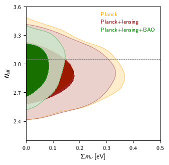
import planckStyle

g = planckStyle.getSinglePlotter(chain_dir = './PLA', ratio=1)

roots = ['base_nnu_mnu_plikHM_TTTEEE_lowl_lowE', 'base_nnu_mnu_plikHM_TTTEEE_lowl_lowE_post_lensing', 'base_nnu_mnu_plikHM_TTTEEE_lowl_lowE_lensing_BAO']
g.settings.solid_contour_palefactor = 0.8
g.plot_2d(roots, 'mnu', 'nnu', filled=True, colors=['orange', 'darkred', 'green'], lims=[0, 0.5, 2.2, 3.6])
g.add_legend(['Planck', 'Planck+lensing', 'Planck+lensing+BAO'], legend_loc='upper right', colored_text=True);
g.add_y_marker(3.046)
g.export('mnu_nnu2.png')

Outputs of the two versions should look like this: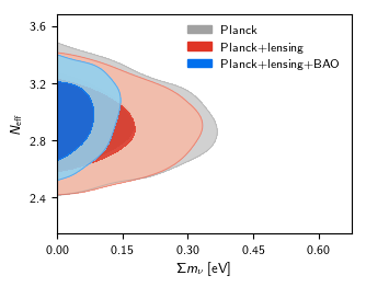

See sample scripts in batch2/outputs, the Plot Gallery and tutorial, and the full GetDist documentation. Note that if you have installed CosmoMC, you don't need to separately install the GetDist python package.

Analysis scripts

The GetDist program can be used to get means, variances, limits etc from all parameters in a chain. The python scripts allow you to do this dynamically, and also offer additional features such as being able to define new derived parameters.

Calculating derived parameters

For simple calculations like finding the mean and variance of new derived parameters you can use the functions in python/chains.py. For example, if you want to calculate the posterior mean and limits for σ₈ Ω_m^0.6 from Planck you could write a python script

import getdist.plots as gplot
g = gplot.getSinglePlotter(chain_dir=r'./PLA')

samples = g.sampleAnalyser.samplesForRoot('base_plikHM_TTTEEE_lowl_lowE_lensing')

p = samples.getParams()

derived = p.sigma8 * p.omegam ** 0.6

print('mean = %s, err = %s'%(samples.mean(derived), samples.std(derived)))
print('95%% limits: %s'%samples.twoTailLimits(derived, 0.95))

Here p.omegam is a vector of parameter values, similar p.sigma8; samples.mean and samples.std sum the samples with the corresponding weights to calculate the result.

See python/getdist/chains.py and python/getdist/mcsamples.py for other functions you can use. Use GetDist or mcsamples.py if you want to reproduce Planck results. The mcsamples module gives you code access to most getdist results, and an MCSamples instance can be obtained from a grid as above, or you can load a chain file directly.

For example if you want to do a power law fit in the variable Ω_m and H₀, you could do

import GetDistPlots as s

g = s.getSinglePlotter(chain_dir=r'./PLA')
samples = g.sampleAnalyser.samplesForRoot('base_plikHM_TTTEEE_lowl_lowE_lensing')

print(samples.PCA(['omegam', 'H0'], 'LL', 'omegam'))

which fits Ω_m and H₀, using log transforms (L), normalized so the exponent of Ω_m is unity (as in GetDist PCA outputs). The output includes

Principle components
PC1 (e-value: 0.008353)
[0.023238]  (\Omega_m/0.315200)^{1.000000}
[0.023238]  (H_0/67.357701)^{2.923650}
          = 1.000005 +- 0.003003

which tells you that Ω_mH₀^2.92 is constrained at the 0.3% level.

Samples can also be loaded directly from single chains, optionally with custom settings, e.g.

import getdist

samples = getdist.loadMCSamples(r'./PLA/base/plikHM_TTTEEE_lowl_lowE_lensing/base_plikHM_TTTEEE_lowl_lowE_lensing', settings={'ignore_rows':0.3})

Or from a grid or list of directories you can find chains automatically e.g.

import planckStyle as s
g = s.getSinglePlotter(chain_dir=['./PLA', './mychains/xxx/'])
samples = g.getSamples('base_plikHM_TTTEEE_lowl_lowE_lensing')

Adding and plotting new derived parameters

You can use the addDerived function of the MCSamples class to add a new parameter to existing chains, which can then be used like any of the original parameters. An example gives the idea (from batch3/outputs/DA-H-BAO.py), which adds a new parameter with name tag 'rsH' which is a function of the original parameters 'Hubble051' and 'rdrag':

p = samples.getParams()
rd_fid = 149.28
rsH = p.Hubble051 * p.rdrag / rd_fid
samples.addDerived(rsH, name='rsH', label=r'H(0.51) (r_{\mathrm{drag}}/r_{\mathrm{drag}}^{\rm fid})\, [{\rm km} \,{\rm s}^{-1}{\rm Mpc}^{-1}]')

After doing this, you can use 'rsH' as you would any of the original parameter names in the chain. If your new parameter has a hard boundary, set the range parameter for addDerived with the [min, max] bounds.

Analysing samples directly

Rather than reading chain files, you can also analyse samples directly, for example using the constructor

 from getdist import mcsamples
 samples = mcsamples.MCSamples(samples=sample_points, loglikes=loglikes, names=names)

where sample_points is a matrix of sample values, names are the parameter names (list of strings), and loglikes is (optionally) an array of corresponding -log(likelihood) values.

Plotting densities

The g.plot_2d (etc) functions will calculate and plot densities from samples, but you can also add densities that are calculated yourself for comparison, e.g.:

from getdist.densities import Density2D
import getdist.plots as gplot
import numpy as np

g = gplot.getSinglePlotter(chain_dir=r'./PLA')

...
xvalues = np.arange(85, 110, 0.3)
yvalues = np.arange(1000, 1500, 4)
x,y = np.meshgrid(xvalues, yvalues)
loglike = my_loglike_func(x,y)
density = Density2D(xvalues,yvalues, np.exp(-loglike / 2))
density.contours = np.exp(-np.array([1.509, 2.4477]) ** 2 / 2)
g.add_2d_contours(root, 'x', 'y', filled=True, density=density)

Other scripts

Multi-purpose use and utility cosmology scripts include

cosmomc_to_camb.py: for converting a dictionary of cosmomc parameters to a python CAMB "CAMBparams" object
extractBestFitCAMB.py: for converting .minimum best-fit file to CAMB input .ini file (not all parameter combinations)
extractBestFitParams.py: for converting .minimum best-fit file to cosmomc input params[xx] settings if you want to fix them
makePerfectForecastDataset.py: a simple old script for simulating perfect fake CMB datasets

Installing Python

Instructions below are for installing python to run things natively on your machine. You could also use CosmoBox.

Python on Windows

See the Python 2.7 download, or install a package like Anaconda (Python 2.7 or 3.4+). Also install matplotlib and PySide standard packages using standard methods (usually included by default in Anaconda), or download builds from here.

Python on a Mac

There are several options, here's one:

Install MacPorts, following the instructions on that page (including installing XCode and command line tools first).

Then from Terminal do

   sudo port install python27
   sudo port select --set python python27
   sudo port install py-matplotlib
   sudo port install py-scipy
   sudo port install py-pyside
   sudo port install texlive-latex-extra
   sudo port install texlive-fonts-recommended
   sudo port install dvipng

Check that python --version says the correct latest version. If not, edit your system path to remove other python installations.

Writing Python

While not needed for GetDist/Cosmomc scripts to run, you may also find an integrated development environment like PyDev or PyCharm useful (they are similar, the latter usually better). This will let you run in one click, check syntax as you type, format nicely, etc.